Blaze Function and the Groove Shadowing Effect

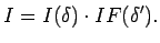
The diffraction function is defined as a product of the blaze function and the grating interference function.

$$I = I(\delta) \cdot IF({\delta}^{\prime}).$$ (20)

The blaze function $I(\delta)$ determines a diffraction envelope and is given by

$$I(\delta) = {\left( \frac{ \sin \delta}{\delta} \right) }^2,$$ (21)

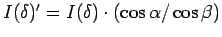
where $\delta$ is the phase difference between the center and edge of a single groove of effective width $s$. The value of $\delta$ is given as,

$$\delta = \frac{\pi}{\lambda} s [ \sin (\alpha - {\theta}_B) + \sin (\beta - {\theta}_B) ],$$ (22)

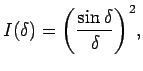
where $\alpha$ is the incident angle, $\beta$ is the diffraction angle, and $\theta _B$ is the blaze angle of the grating. The grating interference function is given by

$$I F = {\left( \frac{\sin N {\delta}^{\prime}}{N \sin {\delta}^{\prime}} \right)}^2,$$ (23)

where ${\delta}^{\prime}$ is the phase difference between the centers of adjacent grooves and $N$ is the number of grooves lighted up by incident beam on the grating. The value of ${\delta}^{\prime}$ is given as follows,

$${\delta}^{\prime} = \frac{\pi}{\lambda} \sigma [\sin \alpha + \sin \beta ],$$ (24)

where $\sigma$ is the groove spacing.

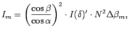
For calculating the integrated intensity of spectral images, we use the peak intensity and effective image width of interference maxima. The peak values of the interference maxima are $N^2$. The effective image width of the $m$th order interference maximum, $\Delta \beta_{m}$, can be considered as a half of the separation of the first minima. The value of $\Delta \beta_m$ is,

$$\Delta {\beta_m} = \frac{\lambda}{N \sigma \cos \beta_m},$$ (25)

where $\beta_{m}$ is the diffraction angle of the $m$th order interference maximum. The integrated intensity of the $m$th order inerference maximum is given by

$$I_{m} = I(\delta) \cdot N^2 \cdot \Delta {\beta_m}$$ (26)

$$= I(\delta) \cdot N^2 \frac{\lambda}{N \sigma \cos \beta_m}.$$ (27)

The form of the blaze function I($\delta$) is dependent on the relation between incident and diffract angles as seen in below.
(a) Case for $\alpha > \beta$
The effective groove width $s$ varies with the incident angle (Figure 8) and can be written as

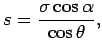$$s = \frac{\sigma \cos \alpha}{\cos \theta},$$ (28)

where $\theta$ is $\alpha - \theta_B$. The blaze function will thus be

$$I(\delta) = sinc^2 \left( \frac{\pi}{\lambda} \frac{ \sigma \cos \alpha}{\cos \theta} [ sin(\alpha -\theta_B) + sin(\beta - \theta_B)] \right).$$ (29)

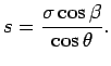
(b) Case for $\alpha < \beta$
In this case, the diffracted beam is vignetted by neighboring grooves (Figure 8) and only the fraction $\cos \beta / \cos \alpha$ contributes to the image (Bottema, 1981). The effective groove width $s$ is determined by the diffracted beam and can be written in the form similar to Eq. 28.

$$s = \frac{\sigma \cos \beta}{\cos \theta}.$$ (30)

The blaze function will be

$$I(\delta) = \frac{\cos \beta}{\cos \alpha} sinc^2 \left( \frac{\p... ...s \beta}{\cos \theta} [sin(\alpha - \theta_B) + sin(\beta - \theta_B)] \right).$$ (31)

The peak values of interference maxima are also smaller than those for the case $\alpha > \beta$. As a result, the integrated intensity will be

$$I_{m} = {\left(\frac{\cos \beta}{\cos \alpha} \right)}^2 \cdot I(\delta)^{\prime} \cdot N^2 \Delta {\beta_m},$$ (32)

where $I(\delta)^{\prime} = I(\delta) \cdot (\cos \alpha / \cos \beta )$.

The effective blaze function ($EBF$) can be written as follows,

$${\rm EBF} = \left\{ \begin{array}{rl} sinc^2 \left( \frac{\p... ...ta - \theta_B ) ] \right) & \mbox{ if $\alpha < \beta$ } \end{array} \right.$$ (33)

where the peak value of the interference maxima are normalized to $N^2$.

Figure 9 shows the EBF when $\theta =$0 and 4 degrees. When $\alpha < \beta$, the amplitude of the EBF is a factor of $(\cos \beta / \cos \alpha)^2$ smaller than that of the EBF for $\alpha \geq \beta$, and the effective width of a single groove gets narrower with increasing $\beta$. As a result, the main envelope of the EBF for $\alpha < \beta$ gets broader for lower amplitudes and the side-lobes are negligible.

The blaze function is affected by polarization. The polarization effect is related to the ratio of wavelength to groove spacing, $\lambda / \sigma$, and the blaze function. The scalar theory can be used as a good approximation when $\lambda / \sigma$ is less than 0.2 (Loewen et al., 1977). For the Littrow case, the ratio can be re-written as follows

$$\frac{\lambda_B}{\sigma} = \frac{2 \sin \theta_B}{m}.$$ (34)

Thus the polarization effect is negligible for high orders. For examples, the ratio is less than 0.2 when $m > 10$ for an R2.00 echelle ( $\theta_B = 63.435$) and an R2.75 echelle ( $\theta_B = 70.0$).

Figure 8: Effective groove widths with incident and diffraction angles.

Figure 9: The effective blaze functions and locations of the interference mazima when (a) $\theta =$ 0 degrees and (b) $\theta =$4 degrees for m $=$ 30 with R2.00 echelle grating . The thin solid lines indicate effective blaze function considered the shadowing effect, which is represented by Eq. 33. The dotted lines indicate blaze functions without shadowing effect. The thick solid vertical lines indicate the interference pattern.The dashed lines indicate the angles when $\alpha = \beta$.